文本作者:劉曉國,Elastic 公司社區佈道師。新加坡國立大學碩士,西北工業大學碩士,曾就職於新加坡科技,康柏電腦,通用汽車,愛立信,諾基亞,Linaro,Ubuntu,Vantiq 等企業。
什麼是 Vega
我們可以在網站 http://vega.github.io/ 找到關於 Vega 的詳細說明。
Vega 聲明式語法是一種可視化數據的強大方法。可視化內容以JSON描述,並使用 HTML5 Canvas 或 SVG 生成交互式視圖。 它是Kibana 6.2中的一項新功能,你現在可以使用 Elasticsearch 數據構建豐富的Vega 和 Vega-Lite 可視化。 因此,讓我們從幾個簡單的示例開始學習 Vega 語言。

首先,打開 Vega編輯器 --- 一種方便的工具來嘗試原始Vega(它沒有 Elasticsearch 定製)。 複製以下代碼,您將看到 "Hello Vega!。 右側面板中的文本。
{
  "$schema": "https://vega.github.io/schema/vega/v3.json",
  "width": 100, "height": 30,
  "background": "#eef2e8",
  "padding": 5,
  "marks": [
    {
      "type": "text",
      "encode": {
        "update": {
          "text":     { "value": "Hello Vega!" },
          "align":    { "value": "center"},
          "baseline": { "value": "middle"},
          "stroke":   { "value": "#A32299" },
          "angle":    { "value": 15 },
          "x":        { "signal": "width/2" },
          "y":        { "signal": "height/2" }
        }
      }
    }
  ]
}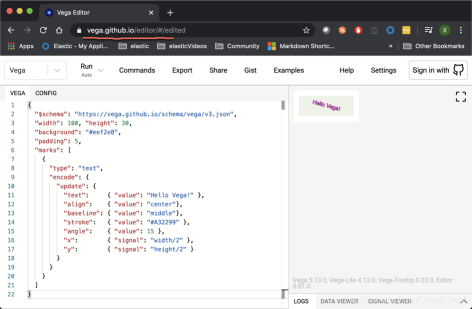
marks 是繪圖圖元的數組,例如文本,線條和矩形。每個標記都有在編碼集(encode-set)中指定的大量參數。在“update”階段,將每個參數設置為常數(值)或計算結果(信號)。對於文本(text)標記,我們指定文本字符串,確保文本相對於給定座標正確放置,旋轉並設置文本顏色。 x和y座標是根據圖形的寬度和高度計算的,將文本放在中間。還有許多其他文本標記參數。還有一個交互式文本標記演示圖,可以嘗試不同的參數值。
$schema 只是所需的 Vega 引擎版本的ID。背景使圖形不透明。width 和 height 設置初始繪圖畫布的大小。在某些情況下,最終的圖形大小可能會根據內容和自動調整大小選項而更改。請注意,Kibana 的默認 autosize 的值是 fit 而不是 pad,因此高度和寬度是可選的。 padding 參數除了寬度和高度外,還在圖形周圍添加了一些空間。
數據驅動圖
我們的下一步是使用矩形標記繪製數據驅動的圖形。 數據部分允許使用硬編碼或URL的多個數據源。 在 Kibana 中,你也可以使用直接 Elasticsearch 查詢。 我們的 vals 數據表有 4 行和 2 列-category 和 count。 我們使用 category 將條形圖放置在 x 軸上,並把 count 設置為條形圖的高度。 請注意,它們的座標 0 在頂部,向下則增加。
{
  "$schema":"https://vega.github.io/schema/vega/v3.json",
  "width": 300, "height": 100,
  "data": [ {
    "name": "vals",
    "values": [
      {"category": 50,  "count": 30},
      {"category": 100, "count": 80},
      {"category": 150, "count": 10},
      {"category": 200, "count": 50}
    ]
  } ],
  "marks": [ {
    "type": "rect",
    "from": { "data": "vals" },
    "encode": {
      "update": {
        "x":     {"field": "category"},
        "width": {"value": 30},
        "y":     {"field": "count"},
        "y2":    {"value": 0}
      }
    }
  } ]
}
rect 標記將 vals 指定為數據源。 每個源數據值(也稱為表格的行或 datum,見下面的例子)繪製一次標記。 與之前的圖不同,x 和 y 參數不是硬編碼的,而是來自基準的字段。
縮放比例 - scaling
scaling 是Vega中最重要但有些棘手的概念之一。 在前面的示例中,屏幕像素座標已硬編碼在數據中。 儘管它使事情變得更簡單,但實際數據幾乎永遠不會以這種形式出現。 取而代之的是,源數據以其自己的單位(例如事件數)進入,並且由圖形決定是否將源值縮放為所需的圖形大小(以像素為單位)。
在此示例中,我們使用線性比例尺---本質上是一個數學函數,用於將源數據域中的值(在此圖中,count 為1000..8000,包括 count = 0)轉換為所需範圍( 在我們的例子中,圖形的高度為0..99)。 在 y 和 y2 參數中都添加 “scale”:“yscale” 使用 yscale 定標器將 count 轉換為屏幕座標(0變為99,而8000-源數據中的最大值-變為0)。 請注意,height range參數是一種特殊情況,將值翻轉以使 0 出現在圖形的底部.
{
  "$schema":"https://vega.github.io/schema/vega/v3.json",
  "width": 400, "height": 100,
  "data": [ {
    "name": "vals",
    "values": [
      {"category": 50,  "count": 3000},
      {"category": 100, "count": 8000},
      {"category": 150, "count": 1000},
      {"category": 200, "count": 5000}
    ]
  } ],
 "scales": [
    {
      "name": "yscale",
      "type": "linear",
      "zero": true,
      "domain": {"data": "vals", "field": "count"},
      "range": "height"
    }
  ],
  "marks": [ {
    "type": "rect",
    "from": { "data": "vals" },
    "encode": {
      "update": {
        "x":     {"field": "category"},
        "width": {"value": 30},
        "y":     {"scale": "yscale", "field": "count"},
        "y2":    {"scale": "yscale", "value": 0}
      }
    }
  } ]
}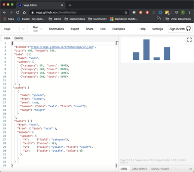
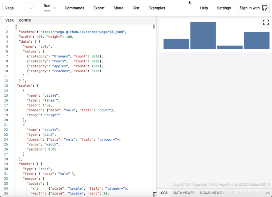
Band scaling
對於我們的教程,我們將需要15種以上的 Vega scale 類型中的另一種---band scale。 當我們有一組值(如類別)需要使用band表示時,將使用此比例尺,每個帶佔據圖形總寬度的相同比例寬度。 在此,帶比例為4個唯一類別中的每個類別賦予相同的比例寬度(大約400/4,在條之間和兩端減去5%的填充)。 {"scale":"xscale","band":1} 獲取標記的 width 參數的樂隊寬度的100%。
{
  "$schema":"https://vega.github.io/schema/vega/v3.json",
  "width": 400, "height": 100,
  "data": [ {
    "name": "vals",
    "values": [
      {"category": "Oranges", "count": 3000},
      {"category": "Pears",   "count": 8000},
      {"category": "Apples",  "count": 1000},
      {"category": "Peaches", "count": 5000}
    ]
  } ],
 "scales": [
    {
      "name": "yscale",
      "type": "linear",
      "zero": true,
      "domain": {"data": "vals", "field": "count"},
      "range": "height"
    },
    {
      "name": "xscale",
      "type": "band",
      "domain": {"data": "vals", "field": "category"},
      "range": "width",
      "padding": 0.05
    }
  ],
  "marks": [ {
    "type": "rect",
    "from": { "data": "vals" },
    "encode": {
      "update": {
        "x":     {"scale": "xscale", "field": "category"},
        "width": {"scale": "xscale", "band": 1},
        "y":     {"scale": "yscale", "field": "count"},
        "y2":    {"scale": "yscale", "value": 0}
      }
    }
  }
 ]
}
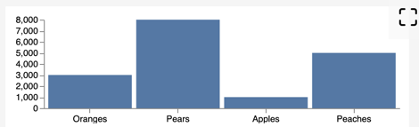
軸
沒有軸標籤,典型的圖形就不會完整。 軸定義使用我們之前定義的比例尺,因此添加它們就像通過其名稱引用比例尺並指定放置側一樣簡單。 將此代碼作為頂級元素添加到最後一個代碼示例中。
"axes": [
    {"scale": "yscale", "orient": "left"},
    {"scale": "xscale", "orient": "bottom"}
 ],
{
"$schema":"https://vega.github.io/schema/vega/v3.json",
"width": 400, "height": 100,
"data": [ {
"name": "vals",
"values": [
{"category": "Oranges", "count": 3000},
{"category": "Pears", "count": 8000},
{"category": "Apples", "count": 1000},
{"category": "Peaches", "count": 5000}
]
} ],
"scales": [
{
"name": "yscale",
"type": "linear",
"zero": true,
"domain": {"data": "vals", "field": "count"},
"range": "height"
},
{
"name": "xscale",
"type": "band",
"domain": {"data": "vals", "field": "category"},
"range": "width",
"padding": 0.05
}
],
"marks": [ {
"type": "rect",
"from": { "data": "vals" },
"encode": {
"update": {
"x": {"scale": "xscale", "field": "category"},
"width": {"scale": "xscale", "band": 1},
"y": {"scale": "yscale", "field": "count"},
"y2": {"scale": "yscale", "value": 0}
}
}
}
],
"axes": [
{"scale": "yscale", "orient": "left"},
{"scale": "xscale", "orient": "bottom"}
]
}
數據轉換和條件
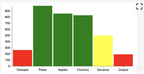
數據通常需要進行其他操作才能用於繪圖。 Vega 提供了許多轉換來幫助你。 讓我們使用最常見的公式轉換為每個源數據動態添加一個隨機 count 字段。 另外,在此圖中,我們將操縱條的填充顏色,如果該值小於333,則將其變為紅色;如果該值小於666,則將其變為黃色;如果該值大於666,則將其變為綠色。請注意,可能是 而是使用比例尺將源數據的域映射到顏色集或配色方案。
{
  "$schema":"https://vega.github.io/schema/vega/v3.json",
  "width": 400, "height": 200,
  "data": [ {
    "name": "vals",
    "values": [
      {"category": "Oranges"},
      {"category": "Pears"},
      {"category": "Apples"},
      {"category": "Peaches"},
      {"category": "Bananas"},
      {"category": "Grapes"}
    ],
    "transform": [
      {"type": "formula", "as": "count", "expr": "random()*1000"}
    ]
  } ],
 "scales": [
    {
      "name": "yscale",
      "type": "linear",
      "zero": true,
      "domain": {"data": "vals", "field": "count"},
      "range": "height"
    },
    {
      "name": "xscale",
      "type": "band",
      "domain": {"data": "vals", "field": "category"},
      "range": "width",
      "padding": 0.05
    }
  ],
  "axes": [
    {"scale": "yscale", "orient": "left"},
    {"scale": "xscale", "orient": "bottom"}
  ],
  "marks": [ {
    "type": "rect",
    "from": { "data": "vals" },
    "encode": {
      "update": {
        "x":     {"scale": "xscale", "field": "category"},
        "width": {"scale": "xscale", "band": 1},
        "y":     {"scale": "yscale", "field": "count"},
        "y2":    {"scale": "yscale", "value": 0},
        "fill":  [
          {"test": "datum.count < 333", "value": "red"},
          {"test": "datum.count < 666", "value": "yellow"},
          {"value": "green"}
        ]
      }
    }
  } ]
}
在 Kibana 中使用 Vega
在上面,我們在 Vega 編輯器中,實踐了一把。我們現在在 Kibana 中來看看是啥樣的。
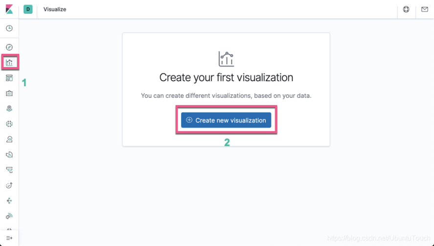
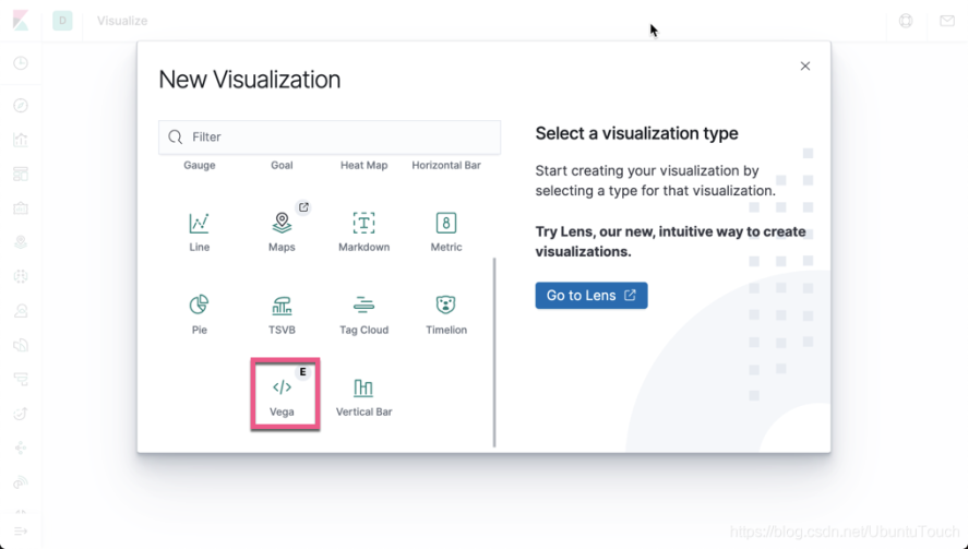
點擊上面的 Create new visualization 按鈕:
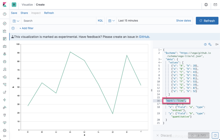
我們使用如下的例子:
{
 "$schema": "https://vega/github.io/schema/vega-lite/v2.json",
  "data": {
    "values": [
      {"a": "A", "b": 28},
      {"a": "B", "b": 55},
      {"a": "C", "b": 43},
      {"a": "D", "b": 91},
      {"a": "E", "b": 81},
      {"a": "F", "b": 53},
      {"a": "G", "b": 19},
      {"a": "H", "b": 87},
      {"a": "I", "b": 52}
    ]
  },
  "mark": "bar",
  "encoding": {
    "x": {"field": "a", "type": "ordinal"},
    "y": {"field": "b", "type": "quantitative"}
  }
}
我們可以把上面的 mark 改為 line:
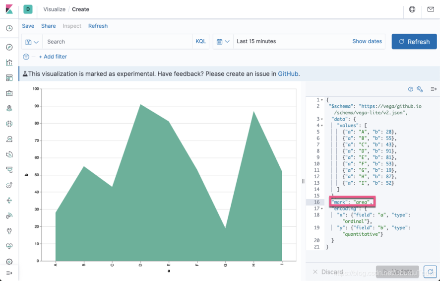
我們可以把上面的 mark 改為 area:
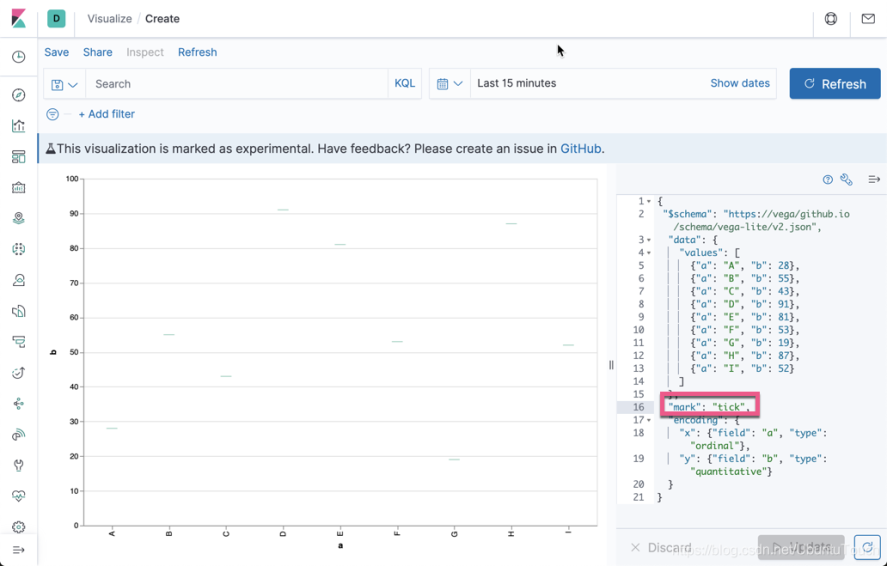
我們可以把上面的 mark 改為 tick:
我們可以把上面的 mark 改為 point

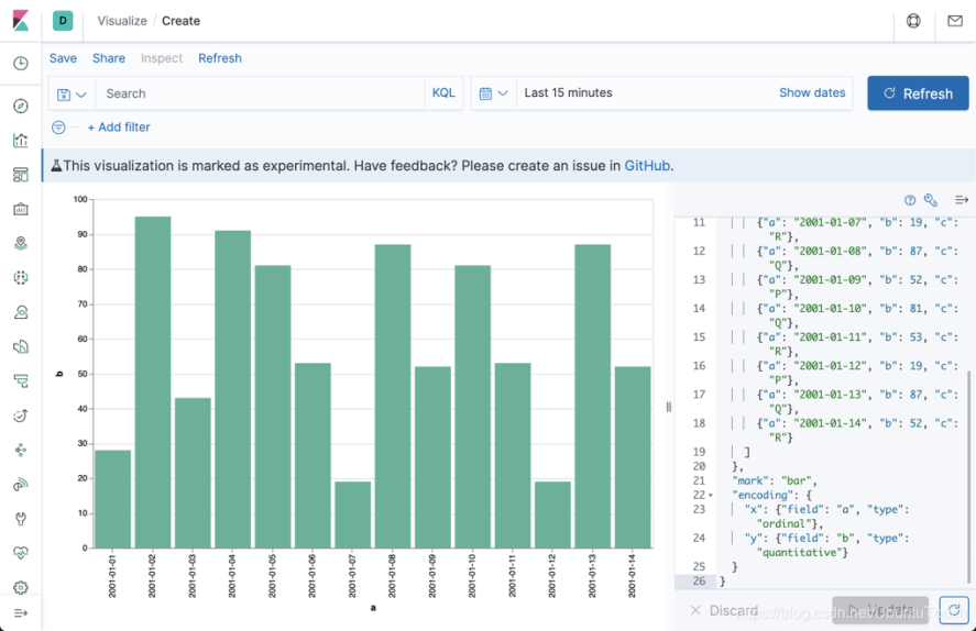
我們再接著使用如下的數據:
{
 "$schema": "https://vega/github.io/schema/vega-lite/v2.json",
  "data": {
    "values": [
      {"a": "2001-01-01", "b": 28, “c": "P"},
      {"a": "2001-01-02", "b": 95, "c": "Q"},
      {"a": "2001-01-03", "b": 43, "c": "R"},
      {"a": "2001-01-04", "b": 91, "c": "Q"},
      {"a": "2001-01-05", "b": 81, "c": "P"},
      {"a": "2001-01-06", "b": 53, "c": "P"},
      {"a": "2001-01-07", "b": 19, "c": "R"},
      {"a": "2001-01-08", "b": 87, "c": "Q"},
      {"a": "2001-01-09", "b": 52, "c": "P"},
      {"a": "2001-01-10", "b": 81, "c": "Q"},
      {"a": "2001-01-11", "b": 53, "c": "R"},
      {"a": "2001-01-12", "b": 19, "c": "P"},
      {"a": "2001-01-13", "b": 87, "c": "Q"},
      {"a": "2001-01-14", "b": 52, "c": "R"}
    ]
  },
  "mark": "bar",
  "encoding": {
    "x": {"field": "a", "type": "ordinal"},
    "y": {"field": "b", "type": "quantitative"}
  }
}
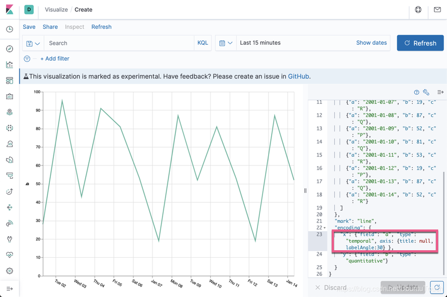
我們再接著修改:
{
 "$schema": "https://vega/github.io/schema/vega-lite/v2.json",
  "data": {
    "values": [
      {"a": "2001-01-01", "b": 28, “c": "P"},
      {"a": "2001-01-02", "b": 95, "c": "Q"},
      {"a": "2001-01-03", "b": 43, "c": "R"},
      {"a": "2001-01-04", "b": 91, "c": "Q"},
      {"a": "2001-01-05", "b": 81, "c": "P"},
      {"a": "2001-01-06", "b": 53, "c": "P"},
      {"a": "2001-01-07", "b": 19, "c": "R"},
      {"a": "2001-01-08", "b": 87, "c": "Q"},
      {"a": "2001-01-09", "b": 52, "c": "P"},
      {"a": "2001-01-10", "b": 81, "c": "Q"},
      {"a": "2001-01-11", "b": 53, "c": "R"},
      {"a": "2001-01-12", "b": 19, "c": "P"},
      {"a": "2001-01-13", "b": 87, "c": "Q"},
      {"a": "2001-01-14", "b": 52, "c": "R"}
    ]
  },
  "mark": "line",
  "encoding": {
    "x": {"field": "a", "type": "temporal", axis: {title: null, labelAngle:30} },
    "y": {"field": "b", "type": "quantitative"}
  }
}
在這裡,我們去到上面 x 軸上顯示的 "a",因為我們已經有時間的標識了。同時,我們把時間標籤傾斜30度。
我們再接著修改數據:
{
 "$schema": "https://vega/github.io/schema/vega-lite/v2.json",
  "data": {
    "values": [
      {"a": "2001-01-01", "b": 28, “c": "P"},
      {"a": "2001-01-02", "b": 95, "c": "Q"},
      {"a": "2001-01-03", "b": 43, "c": "R"},
      {"a": "2001-01-04", "b": 91, "c": "Q"},
      {"a": "2001-01-05", "b": 81, "c": "P"},
      {"a": "2001-01-06", "b": 53, "c": "P"},
      {"a": "2001-01-07", "b": 19, "c": "R"},
      {"a": "2001-01-08", "b": 87, "c": "Q"},
      {"a": "2001-01-09", "b": 52, "c": "P"},
      {"a": "2001-01-10", "b": 81, "c": "Q"},
      {"a": "2001-01-11", "b": 53, "c": "R"},
      {"a": "2001-01-12", "b": 19, "c": "P"},
      {"a": "2001-01-13", "b": 87, "c": "Q"},
      {"a": "2001-01-14", "b": 52, "c": "R"}
    ]
  },
  "mark": "line",
  "encoding": {
    "x": {"field": "a", "type": "temporal", axis: {title: null, labelAngle:30} },
    "y": {"field": "b", "type": "quantitative"},
    "color": {"field": "c", "type": "nominal"}
  }
}
在這裡,我們在 encoding 裡添加一個叫做 color 的項:

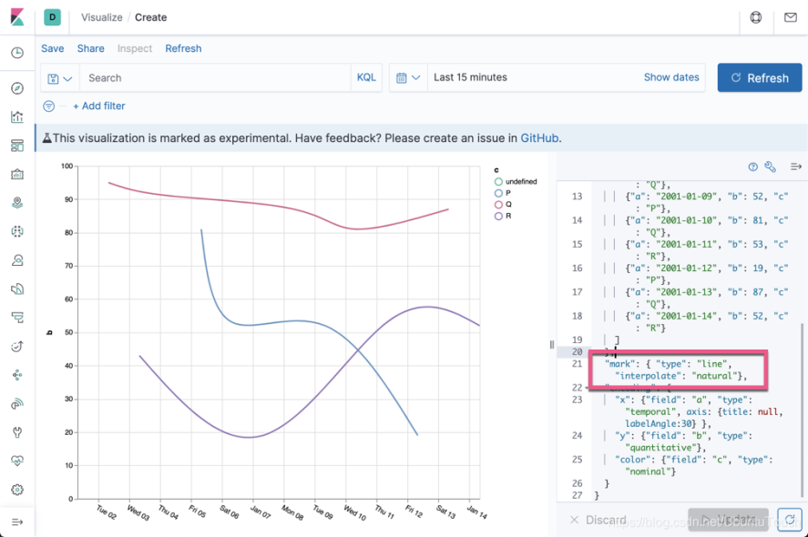
上面的線感覺特別粗糙,我們可以進行插值。我們把 mark 這行修改為:
"mark": { "type": "line", "interpolate": "natural"},
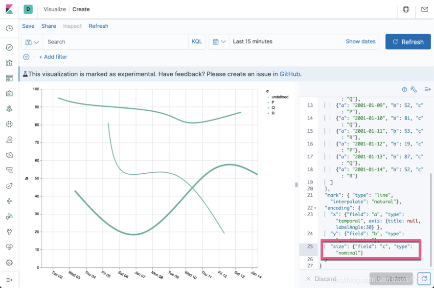
我們也可以通過線的粗細來表示不同的類:
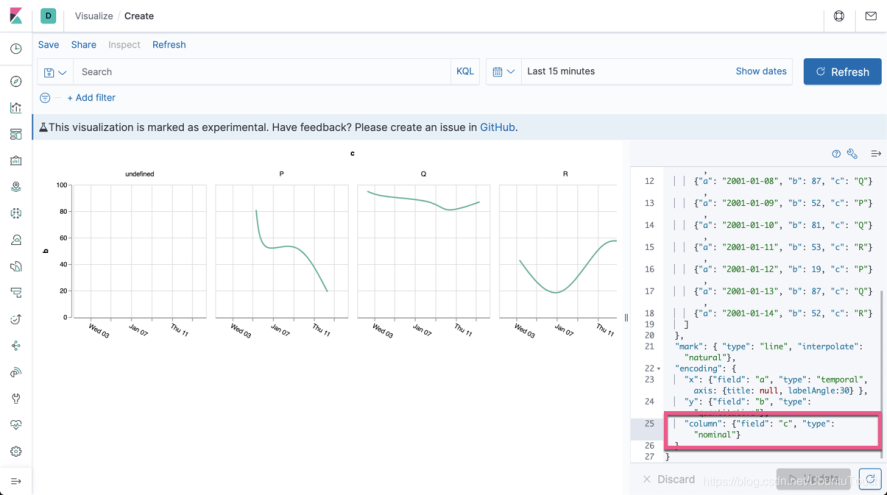
我們也可以用不同 graph 來分別表達:
針對顏色,我們可以可以設置不同的 color scheme:

使用 Elasticsearch 和 Kibana 進行動態數據
現在您已經瞭解了基礎知識,讓我們嘗試使用一些隨機生成的 Elasticsearch 數據創建基於時間的折線圖。 這與你在 Kibana 中創建新的 Vega 圖時最初看到的內容相似,不同之處在於,我們將使用 Vega 語言而不是 Vega-Lite 的 Kibana 默認值(Vega的簡化高級版本)。
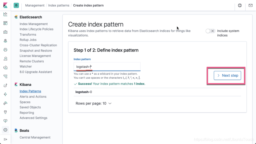
創建隨機的 Logstash 日誌數據
如果你還不知道如何生成這些隨機的數據,請參閱我之前的文章 “Logstash:運用 makelogs 創建測試日誌”。我們使用如下的命令來生成20000個數據。我們首先為我們剛才生成的一個叫做 logstash-0 的索引創建一個 index pattern:
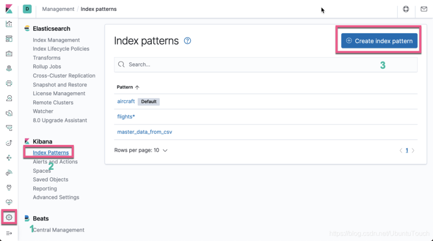
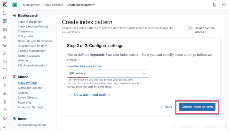
這樣我們就生產了我們想要的 index pattern。
我們可以做一些簡單的查詢,比如:
<p style="text-align:center"><img src="https://ucc.alicdn.com/pic/developer-ecology/998ee5af1c634cae84df66686c318e20.png" width="500" height="300" alt="深圳"/></p>
我們可以看到有一個timestamp 及文件的擴展名類型 extension。請注意上面的 hits.hits。這個也是我們在下面想要用到的。
運用 Vega 來展示數據
在上面的 Vega 實驗中,我們對 values 數據進行硬編碼,而不是使用 url 進行實際查詢。 這樣,我們可以繼續在不支持 Kibana Elasticsearch 查詢的 Vega 編輯器中進行測試。 如果你將值替換為url部分,則該圖將在 Kibana 內部變得完全動態,如下所示。
{
"$schema": "https://vega/github.io/schema/vega-lite/v2.json",
data: {
"url": {
"index": "logstash-*",
"body": {
"size": 100,
"_source": ["@timestamp", "extension"]
}
}
"format":{"property":"hits.hits"}
},
"transform": [
{
"calculate": "toDate(datum._source['@timestamp'])", "as": "time"
},
{
"calculate": "datum._source.extension", "as": "ext"
}
],
"mark": "circle",
"encoding": {
}
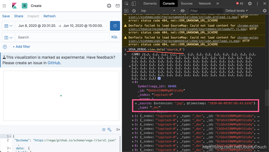
}在上面,我們替換之前 values 的硬編碼,取而代之的是查詢 logstash-* 索引。我們先查詢 100 個數據,同時,我們只對 hits.hits 的內容感興趣。另外我們通過 transform 把@timestamp 轉換為 time,extension 轉換為 ext。運行 Vega:

上面顯示的是一個點,這是因為我們還沒對 x 及 y 軸做任何的設置。
我們可以在瀏覽器中的 Developer Tools 裡進行查看:
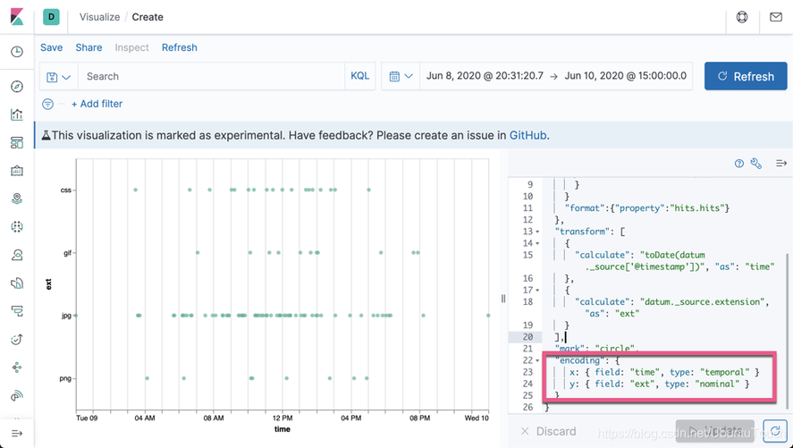
接下來我們配置 x 及 y 軸:
{
 "$schema": "https://vega/github.io/schema/vega-lite/v2.json",
  data:  {
   "url": {
      "index": "logstash-*",
      "body": {
        "size": 100,
        "_source": ["@timestamp", "extension"]
      }
    }
    "format":{"property":"hits.hits"}
  },
  "transform": [
    {
      "calculate": "toDate(datum._source['@timestamp'])", "as": "time"
    },
    {
      "calculate": "datum._source.extension", "as": "ext"
    }
  ],
  "mark": "circle",
  "encoding": {
     x: { field: "time", type: "temporal" }
     y: { field: "ext", type: "nominal" }
  }
}
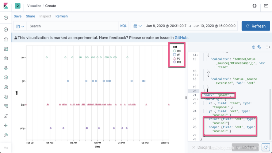
就像我們上面的那樣,我們可以添加顏色及形狀:
{
 "$schema": "https://vega/github.io/schema/vega-lite/v2.json",
  data:  {
   "url": {
      "index": "logstash-*",
      "body": {
        "size": 100,
        "_source": ["@timestamp", "extension"]
      }
    }
    "format":{"property":"hits.hits"}
  },
  "transform": [
    {
      "calculate": "toDate(datum._source['@timestamp'])", "as": "time"
    },
    {
      "calculate": "datum._source.extension", "as": "ext"
    }
  ],
  "mark": "point",
  "encoding": {
     x: { field: "time", type: "temporal" }
     y: { field: "ext", type: "nominal" }
     color: {field: "ext", type: "nominal"}
     shape: {field: "ext", type: "nominal" }
  }
}
目前我們的數據還不能和 search field 相關聯,比如我們搜索 extension:css,但是我們的顯示的圖還是不會變好。另外,當我們選擇右上角的時間選擇時,我們的也不會變化。為了能關聯起來,我們添加如下的兩個字段到 url 中:
      "%context%": true,
      "%timefield%": "@timestamp",
{
"$schema": "https://vega/github.io/schema/vega-lite/v2.json",
data: {
"url": {
"%context%": true,
"%timefield%": "@timestamp",
"index": "logstash-*",
"body": {
"size": 100,
"_source": ["@timestamp", "extension"]
}
}
"format":{"property":"hits.hits"}
},
"transform": [
{
"calculate": "toDate(datum._source['@timestamp'])", "as": "time"
},
{
"calculate": "datum._source.extension", "as": "ext"
}
],
"mark": "point",
"encoding": {
x: { field: "time", type: "temporal" }
y: { field: "ext", type: "nominal" }
color: {field: "ext", type: "nominal"}
shape: {field: "ext", type: "nominal" }
}
}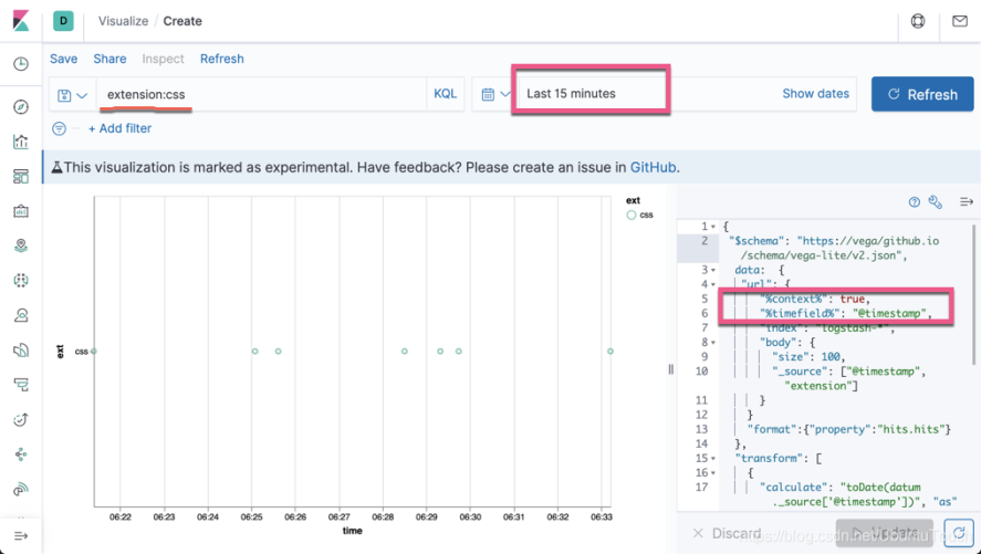
通過上面的關聯,我們可以看出來,我們少了很多的數據,通過搜索 extension:css。
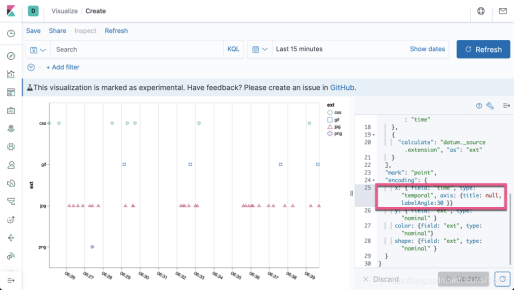
我們發現 x 軸的 time 是沒有啥用處。我們可以去掉它。我們同時旋轉時間的標籤30度:
{
 "$schema": "https://vega/github.io/schema/vega-lite/v2.json",
  data:  {
   "url": {
      "%context%": true,
      "%timefield%": "@timestamp",
      "index": "logstash-*",
      "body": {
        "size": 100,
        "_source": ["@timestamp", "extension"]
      }
    }
    "format":{"property":"hits.hits"}
  },
  "transform": [
    {
      "calculate": "toDate(datum._source['@timestamp'])", "as": "time"
    },
    {
      "calculate": "datum._source.extension", "as": "ext"
    }
  ],
  "mark": "point",
  "encoding": {
     x: { field: "time", type: "temporal", axis: {title: null, labelAngle:30 }}
     y: { field: "ext", type: "nominal" }
     color: {field: "ext", type: "nominal"}
     shape: {field: "ext", type: "nominal" }
  }
}
接下來,我們嘗試使用更多的數據,並使用 Elasticsearch 所提供的強大的 aggregation 功能。首先我們在 Kibana 中做如下的搜索:
GET logstash-0/_search
{
  "size": 0,
  "aggs": {
    "table": {
      "composite": {
        "size": 10000,
        "sources": [
          {
            "time": {
              "date_histogram": {
                "field": "@timestamp",
                "calendar_interval": "1d"
              }
            }
          },
          {
            "ext": {
              "terms": {
                "field": "extension.keyword"
              }
            }
          }
        ]
      }
    }
  }
}
它顯示的結果為:
{
  "took" : 6,
  "timed_out" : false,
  "_shards" : {
    "total" : 1,
    "successful" : 1,
    "skipped" : 0,
    "failed" : 0
  },
  "hits" : {
    "total" : {
      "value" : 10000,
      "relation" : "gte"
    },
    "max_score" : null,
    "hits" : [ ]
  },
  "aggregations" : {
    "table" : {
      "after_key" : {
        "time" : 1591920000000,
        "ext" : "jpg"
      },
      "buckets" : [
        {
          "key" : {
            "time" : 1591574400000,
            "ext" : "css"
          },
          "doc_count" : 159
        },
        {
          "key" : {
            "time" : 1591574400000,
            "ext" : "gif"
          },
          "doc_count" : 71
        },
        {
          "key" : {
            "time" : 1591574400000,
            "ext" : "jpg"
          },
          "doc_count" : 592
        },
        {
          "key" : {
            "time" : 1591574400000,
            "ext" : "php"
          },
          "doc_count" : 25
        },
        {
          "key" : {
            "time" : 1591574400000,
            "ext" : "png"
          },
          "doc_count" : 80
        },
        {
          "key" : {
            "time" : 1591660800000,
            "ext" : "css"
          },
          "doc_count" : 1043
        },
        {
          "key" : {
            "time" : 1591660800000,
            "ext" : "gif"
          },
          "doc_count" : 458
        },
        {
          "key" : {
            "time" : 1591660800000,
            "ext" : "jpg"
          },
          "doc_count" : 4365
        },
        {
          "key" : {
            "time" : 1591660800000,
            "ext" : "php"
          },
          "doc_count" : 234
        },
        {
          "key" : {
            "time" : 1591660800000,
            "ext" : "png"
          },
          "doc_count" : 598
        },
        {
          "key" : {
            "time" : 1591747200000,
            "ext" : "css"
          },
          "doc_count" : 1048
        },
        {
          "key" : {
            "time" : 1591747200000,
            "ext" : "gif"
          },
          "doc_count" : 427
        },
        {
          "key" : {
            "time" : 1591747200000,
            "ext" : "jpg"
          },
          "doc_count" : 4301
        },
        {
          "key" : {
            "time" : 1591747200000,
            "ext" : "php"
          },
          "doc_count" : 199
        },
        {
          "key" : {
            "time" : 1591747200000,
            "ext" : "png"
          },
          "doc_count" : 639
        },
        {
          "key" : {
            "time" : 1591833600000,
            "ext" : "css"
          },
          "doc_count" : 936
        },
        {
          "key" : {
            "time" : 1591833600000,
            "ext" : "gif"
          },
          "doc_count" : 340
        },
        {
          "key" : {
            "time" : 1591833600000,
            "ext" : "jpg"
          },
          "doc_count" : 3715
        },
        {
          "key" : {
            "time" : 1591833600000,
            "ext" : "php"
          },
          "doc_count" : 192
        },
        {
          "key" : {
            "time" : 1591833600000,
            "ext" : "png"
          },
          "doc_count" : 579
        },
        {
          "key" : {
            "time" : 1591920000000,
            "ext" : "jpg"
          },
          "doc_count" : 6
        }
      ]
    }
  }
}
請注意上面的數據結構,在接下來的 Vega 中將被採用。
重新書寫我們的 Vega:
{
"$schema": "https://vega/github.io/schema/vega-lite/v2.json",
data: {
"url": {
"%context%": true,
"%timefield%": "@timestamp",
"index": "logstash-*",
"body": {
"size": 0,
"aggs": {
"table": {
"composite": {
"size": 10000,
"sources": [
{
"time": {
"date_histogram": {
"field": "@timestamp",
"interval": {%autointerval%:400}
}
}
},
{
"ext": {
"terms": {
"field": "extension.keyword"
}
}
}
]
}
}
}
}
}
"format":{"property":"aggregations.table.buckets"}
},
"transform": [
{
"calculate": "toDate(datum.key.time)", "as": "time"
},
{
"calculate": "datum.key.ext", "as": "ext"
}
],
"mark": "area",
"encoding": {
x: {
field: "time",
type: "temporal"
},
y: {
axis: {title: "Document count"}
field: "doc_count",
type: "quantitative"
}
color: {field: "ext", type: "nominal"}
}
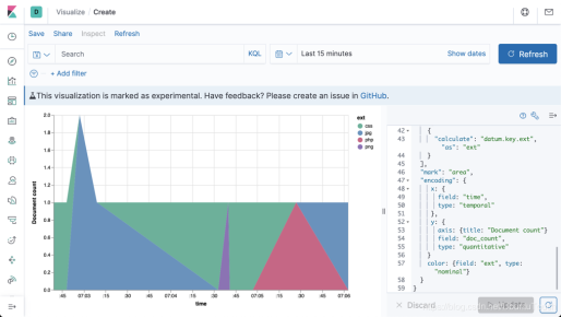
}請注意上面的有些地方已經根據 aggregation 的結果做了相應的調整。展示的結果是:
最後,我們取消 x 軸上的 time,並且,我們把所有的數據都 stack 起來:
{
 "$schema": "https://vega/github.io/schema/vega-lite/v2.json",
  data:  {
   "url": {
      "%context%": true,
      "%timefield%": "@timestamp",
      "index": "logstash-*",
      "body": {
        "size": 0,
        "aggs": {
          "table": {
            "composite": {
              "size": 10000,
              "sources": [
                {
                  "time": {
                    "date_histogram": {
                      "field": "@timestamp",
                      "interval": {%autointerval%:400}
                    }
                  }
                },
                {
                  "ext": {
                    "terms": {
                      "field": "extension.keyword"
                    }
                  }
                }
              ]
            }
          }
        }
      }
    }
    "format":{"property":"aggregations.table.buckets"}
  },
  "transform": [
    {
      "calculate": "toDate(datum.key.time)", "as": "time"
    },
    {
      "calculate": "datum.key.ext", "as": "ext"
    }
  ],
  "mark": "area",
  "encoding": {
     x: {
       field: "time",
       type: "temporal",
       axis: {title: null}
     },
     y: {
       axis: {title: "Document count"},
       field: "doc_count",
       type: "quantitative" ,
       stack: normalize
    }
    color: {field: "ext", type: "nominal"}
  }
}
我們是使用 makelogs 拉絲生成的數據。它生成的數據是在一天內的,並且是平均的。從上面,我們可以看出來各個文件的比例。
好了。今天的文章就寫到這裡。希望大家也學到了一些東西。
更多資料:
【1】https://vega.github.io/vega-lite/tutorials/getting_started.html
【2】https://www.elastic.co/blog/getting-started-with-vega-visualizations-in-kibana
【3】 https://www.elastic.co/guide/en/kibana/master/vega-graph.html
【4】https://vega.github.io/vega/examples/
【5】https://vega.github.io/vega-lite/examples/